Getting started
Installation
git clone https://github.com/tomboulier/SIES.git
cd SIES
pip install -e .
For development (tests, linting, notebooks):
pip install -e .[dev]
A complete identification experiment
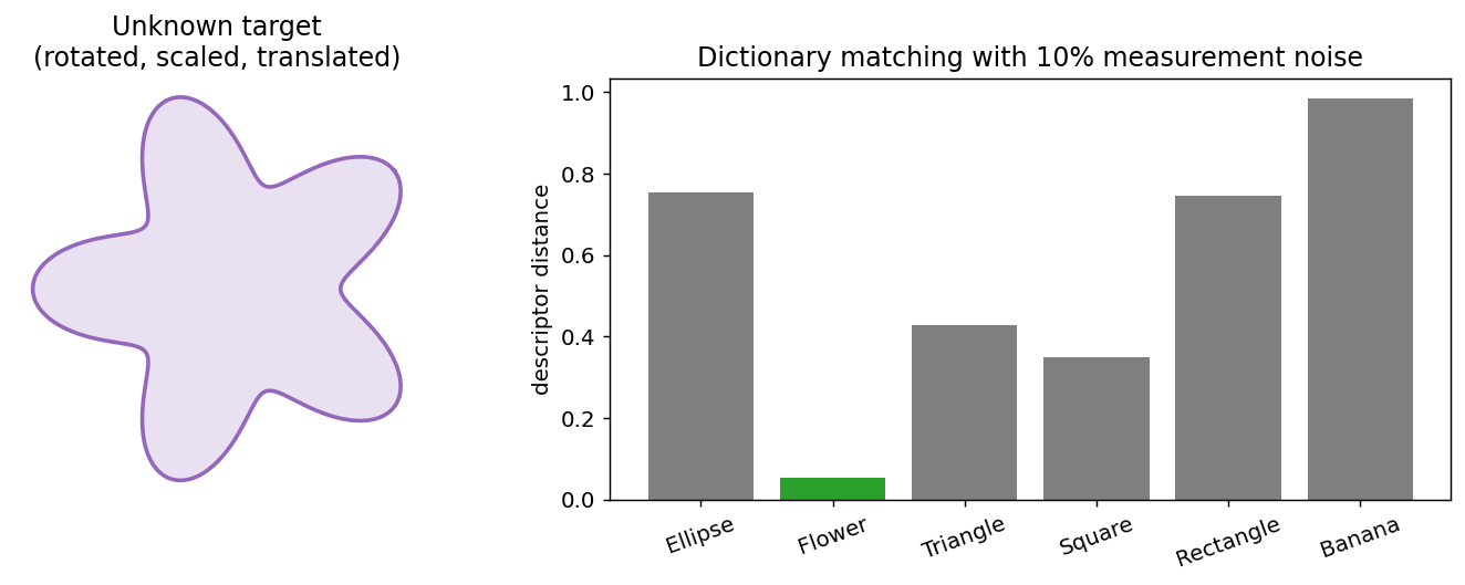
This walkthrough reproduces the dictionary matching experiment of the FoCM 2014 paper: an unknown target is illuminated by point sources, and identified among a dictionary of reference shapes.
1. Build a dictionary of shapes
import numpy as np
from sies.shapes import Ellipse, Flower, Rectangle, Triangle
from sies.dictionary import ShapeDictionary

nb_points = 256  # boundary discretization
shapes = [
    Ellipse(1.0, 0.5, nb_points),
    Flower(1.0, 1.0, nb_points),
    Triangle(1.0, np.pi / 3, nb_points),
    Rectangle(1.0, 1.0, nb_points),
]
dico = ShapeDictionary.build(shapes, cnd=3.0, order=5)
ShapeDictionary.build computes the theoretical CGPT of each shape by solving
boundary integral equations, then converts it into descriptors invariant under
translation, rotation and scaling.
2. Simulate measurements of an unknown target
The target is a transformed dictionary element — the identification must succeed regardless of its position, orientation and size:
from sies.acquisition import Coincided
from sies.pde import ConductivityR2

target = (Flower(1.0, 1.0, nb_points).rotate(0.2 * np.pi) * 0.75) + np.array([0.25, 0.25])

cfg = Coincided(np.zeros(2), radius=1.5, nb_src=100)
pde = ConductivityR2(target, cnd=3.0, pmtt=0.0, cfg=cfg)

data = pde.simulate_data(freqs=0.0)
noisy = pde.add_white_noise(data, level=0.05)  # 5% noise
3. Reconstruct the CGPT and identify the shape
from sies.dictionary import ShapeDescriptor

result = pde.reconstruct_cgpt_analytic(noisy.msr_noisy[0], order=5)
descriptor = ShapeDescriptor.from_cgpt(result.cgpt[0])

errors, ranking = dico.match(descriptor, order=3)
print(dico.identify(descriptor, order=3))  # "Flower"
Tracking a moving target
The same machinery tracks a moving target whose CGPT is known, using an Extended Kalman Filter:
from sies.asymptotics import contrast, theoretical_cgpt
from sies.tracking import (
    CGPTObservation, ExtendedKalmanFilter, simulate_target_path, target_dynamics,
)

shape = Ellipse(1.0, 0.5, 128) * 0.2
cgpt = theoretical_cgpt(shape, contrast(3.0), 2).real

cfg = Coincided(np.zeros(2), 3.0, 30)
pde = ConductivityR2(shape, 3.0, 0.0, cfg)
src_matrix, rcv_matrix = pde.make_linear_operator(2)
observation = CGPTObservation(src_matrix, rcv_matrix, cgpt)

dt, nb_steps = 0.1, 100
state_matrix, process_cov, _ = target_dynamics(dt, std_acc=0.5, std_acc_angle=0.2)
ekf = ExtendedKalmanFilter(
    state_matrix, process_cov, observation, observation.jacobian,
    observation_cov=1e-4 * np.eye(cfg.data_dim),
)
# estimates = ekf.run(measurements, initial_state)
![]()
Going further
- The notebooks are interactive, reproducible versions of these experiments.
- The mathematical background page summarizes the theory.
- The API reference documents every public function.